1. VS C++ 2019
2. Nvidia Cuda Toolkit 12.1
3. SDL2
4. Whisper.cpp Source
5. Git
6. CMake
If your visual studio did not detected by the Nvidia Toolkit make sure to copy following directory content to the next one manually. You may need to adjust the path depending on your specific VS version.
C:\Program Files\NVIDIA GPU Computing Toolkit\CUDA\v12.1\extras\visual_studio_integration\MSBuildExtensions
C:\Program Files (x86)\Microsoft Visual Studio\2019\BuildTools\MSBuild\Microsoft\VC\v160\BuildCustomizations
You need to also install SDL2, this only required for streaming option. You have to install the SDL2, building locally and reference locally will cause the whisper compile process to fail.
cd SDL2
cmake -B build
cmake --build build --config Release --target installgit clone https://github.com/ggml-org/whisper.cpp.git
cd whisper.cpp
cmake -B build -DWHISPER_SDL2=ON -DGGML_CUDA=1 -DWHISPER_BUILD_EXAMPLES=1 -DSDL2_DIR="SDL2/" -DCMAKE_PREFIX_PATH="SDL2/cmake"This is the golden formula in the speech recognition.

The argmax function means find the value of w that makes p(x|w) maximum. Here x is observation acoustic signal. So basically we compute all possible sequence and then for each one of them calculate the possibility of seeing such an acoustic signal. This is a very computation intensive process but by using HMM and CTC we try to minimize searching space. The process of guessing the correct sequence is called decoding in the speech recognition research field.
HMM is just bunch of states that transition from one state to the other. These would be called on every emitting transitions and all of them can be expressed in a matrix that would be called transition matrix.

| • Occupation counts: | .occs It’s the per-transition-id occupation counts. They are rarely needed. e.g. might be used somewhere in the basis-fMLLR scripts. |
| • FMLLR: | An acoustic feature extraction technique like MFCC but with focus on multi-speaker adaptation. |
| • Beam: | Cutoff would be Best Cost–Beam (Around 10 to 16) |
| • Deterministic FST: | A FST that each state has at most one transition with any given input label and there are no input eps-labels. |

RNN or CNN, that’s the question. so what should you use?
Let the battle begin
So speech recognition is a very broad task. People use speech recognition to do speech-to-text on videos, a pre-recorded data which you can go back and forth between past and future and optimize the output a couple of times. On the other hand voice control is also a speech recognition task, but you need to do all this speech processing in real time. And within a low latency time manner.
And now comes the big question. Which technologies should you use RNN or CNN? in this post, We’re going to talk about that
so generally, speech waveform data by using a CMVN or MFCC, can be converted to 2D image data and then, from that point is basically an image that you can show to people and people can learn how each word will look like. So, it is basically detecting where exactly the word is happening. And it’s very similar to an object detection task. very similar, but not quite the same. And why is that? So, a lot of times we also have trouble detecting words but we are using the language grammar in the background of our head to predict what exactly the next word would look like. And we’re using that and combining that with the waveform data and then we detect the right word so if you say, a very strange word to people, they will have trouble getting the correct text out of it. But if you teach them a couple of times, and they know that when these words pop up, they will have much less trouble detecting them. So the machine learning community uses the same approach.
In modern speech recognition engines ML engineers first use CNN to capture the features, or at least detect how likely the word is, and then run an RNN in the background as a language model to improve the result. So in the case of voice control, you don’t care about the language model, because there is no language model. You can say whatever word you want, or at least we give you that freedom, and then you just need the text out of the word that you just said.
So in that case there is no use for RNN as there is no language model. And a 1D convolutional network is enough. So it is the same as localization and object detection in classic machine learning. So if you use the same technique as YOLO to move around the convolution layer, around the waveform, and just detect the maximum confidence score on a window, then you can find the exact word happening at that time. The problem is as the number of words increases and increases this technique will become more and more challenging. So you need to develop more mature techniques. And that’s exactly why we introduced HMM. The best technique is to use a hidden Markov model To detect which word is spoken in a certain way and then slide that word over the signal and find out if it’s actually that signal or not. And by using that we can do that alignment. We can do better force alignment, use that data, and also feed it to Hmm, To increase the accuracy and finally, we create this awesome engine with a great amount of accuracy that no one has seen ever before.
So wait for it and Sleep on it.
-log(p_target_class). So basically it only depends on the class that the input data is belonged to. In this case other classes error don’t have any impact on the network loss.slavv – 37 reasons why your neural network-is-not-working
To calculate word level confidence score Kaldi uses a method called MBR Decoding. MBR Decoding is a decoding process that minimize word level error rate (instead of minimizing the whole utterance cost) to calculate the result. This may not give the accurate result but can be use to calculate the confidence score up to some level. Just don’t expect too much as the performance is not well-accurate.
Here are some key concepts:
1. Levenshtein Distance: Levenshtein Distance or Edit Distance compute difference between two sentences. It computes how many words are different between the two. Lets say X and Y are two word sequence shown below. The Levenshtein distance would be 3 where Ɛ represent empty word

To calculate the Levenshtein distance you can use following recursive algorithm where A and B are word sequence with length of N+1

As in all recursive algorithm to decrease amount of duplicate computation Kaldi used the memoization technique and store the above three circumstances in a1, a2 and a3 respectively
2. Forward-Backward Algorithm: Lets say you want to calculate the probability of seeing a waveform(or MFCC features) given a path in a lattice (or on HHM FST). Then the Forward-Backward Algorithm is nothing more than a optimized way to compute this probability.

3. Gamma Calculation: TBA
4. MBR Decoding: TBA
Delta-Delta feature is proposed in 1986 by S. Furui and Hermann Ney in 1990. It’s simply add first and second derivative of cepstrum to the feature vector. By doing that they say it can capture spectral dynamics and improve overall accuracy.
The only problem is that in a discrete signal space getting derivative from the signal increase spontaneous noise level so instead of simple first and second order derivative HTK proposed a differentiation filter. This filter basically is a convoluted low-pass filter on top of discrete signal derivative to smooth out the result and remove unwanted noises. In Fig 1 you can see the result of simple second derivative vs the proposed differentiation filter.
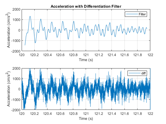
Fig. 1. Plain dervative VS differentiation filter. courtesy of Matlab™
HTK filter for a Delta-Delta feature (order=2, window=2) is a 9 element FIR filter with following coefficient(Θ is window size which is 2 in HTK)

| • Reverberation: | Is the effect of sound bouncing the walls and getting back in a room. The time is roughly between 1 and 2 second in an ordinary room. You can use Sabine equation to do more accurate calculation. |
compressor filter in speech instead of CMVN to normalize in real-time.IEEE ICASSP ’86 – Isolated Word Recognition Based on Emphasized Spectral Dynamics
IEEE ICASSP ’90 – Experiments on mixture-density phoneme-modelling for 1000-word DARPA task
Desh Raj Blog – Award-winning classic papers in ML and NLP
| • Lattices: | Are a graph containing states(nodes) and arcs(edges). which each state represent one 10ms frame |
| • Arcs: | Are start from one state to another state. Each state arcs can be accessed with arc iterator and arcs only retain their next state. each arcs have weight and input and output label. |
| • States: | Are simple decimal number starting from lat.Start(). and goes up to lat.NumStates(). Most of the time start is 0 |
| • Topological Sort: | An FST is topological sorted if the FST can be laid out on a horizontal axis and no arc direction would be from right to left |
| • Note 1: | You can get max state with lat.NumStates() |
| • Note 2: | You can prune lattices by creating dead end path. Dead end path is a path that’s not get end up to the final state. After that fst::connect will trim the FST and get rid of these dead paths |
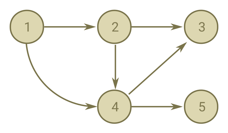
Fig. 1. Topologically Sorted Graph
| • Link: | Same as arc |
| • Token: | Are same as state. They have costs |
| • FrameToks: | A link list that contain all tokens in a single frame |
| • Adaptive Beam: | Used in pruning before creating lattice and through decoding |
| • NEmitting Tokens: | Non Emitting Tokens or NEmitting Tokens are tokens that generate from emitting token in the same frame and have input label = 0 and have acoustic_cost = 0 |
| • Emitting Tokens: | Emitting Tokens are tokens that surpass from a frame to another frame |
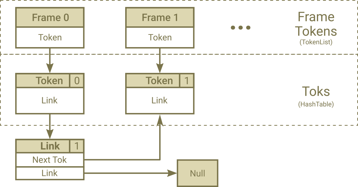
Fig. 1. After First Emitting Nodes Process
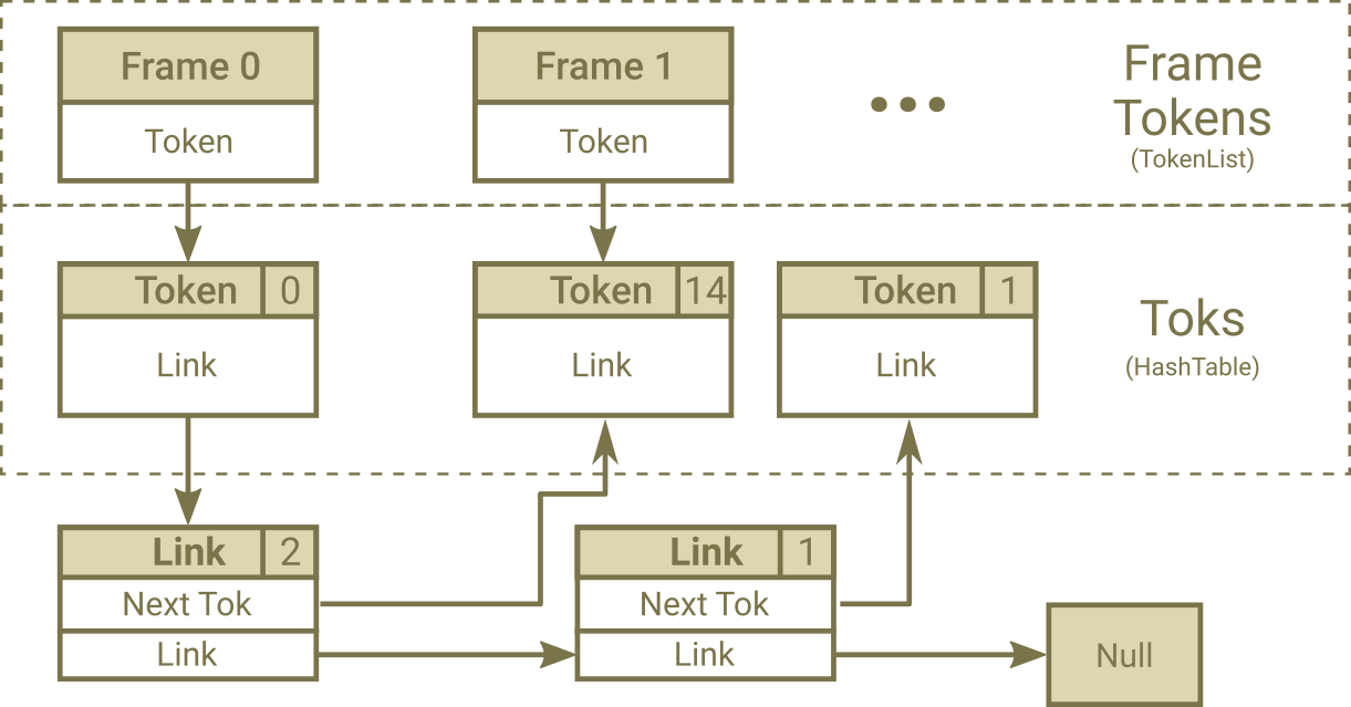
Fig. 2. After Second Emitting Nodes Process
A Simplified Block Diagram of ASR Process in Kaldi

| • Costs: | Are Log Negative Probability, so a higher cost means lower probability. |
| • Frame: | Each 10ms of audio that using MFCC turned into a fixed size vector called a frame. |
| • Beam: | Cutoff would be Best Cost–Beam (Around 10 to 16) |
| • Cutoff: | The maximum cost that all cost higher than this value will not be processed and removed. |
| • Epsilon: | The zero label in FST are called <eps> |
| • Lattices: | Are the same as FSTs, instead each token keeps in a framed based array calledframe_toks. In This way the distance in time between each token will be perceived too. |
| • Rescoring: | A language model scoring system that applied after final state to improve final result by using stronger LM model than n-gram. |
| • HCLG(FST): | The main FST used in the decoding. The iLabel in this FST is TransitionIDs. |
| • Model(MDL): | A model that used to convert sound into acoustic cost and TransitionIDs. |
| • TransitionIDs: | A number that contain information about state and corresponding PDF id. |
| • Emiting States: | States that have pdfs associated with them and emit phoneme. In other word states that have their ilabel is not zero |
| • Bakis Model: | Is a HMM that state transitions proceed from left to right. In a Bakis HMM, no transitions go from a higher-numbered state to a lower-numbered state. |
| • Max Active: | Uses to calculate cutoff to determince maximum number of tokens that will be processed inside emitting process. |
| • Graph Cost: | is a sum of the LM cost, the (weighted) transition probabilities, and any pronunciation cost. |
| • Acoustic Cost: | Cost that is got from the decodable object. |
| • Acoustic Scale: | A floating number that multiply in all Log Likelihood (inside the decodable object). |
 Fig. 1. Demonstration of Finite State Automata vs Lattices, Courtesy of Peter F. Brown

